Note
The objective of this technote is to clarify all the different coordinate systems that are relevant to the operations of the Rubin Observatory Active Optics System, and the transformations between them, which is crucial for the Active Optics Control to work in a coherent way.
1 Introduction
The operations of the Rubin Observatory Active Optics System (AOS) involve the following components,
- M1M3
- M2
- M2 hexapod
- Camera hexapod
- Camera rotator
- ComCam (during commissioning)
- LSSTCam (during commissioning and operations)
Over the years, each component has been under development under their own coordinate system (CS). Sometimes the situation can be even more complicated - A single vendor may be using multiple CSs for different sub-components (for example, mechanical versus optical). There are also inconsistencies between various engineering models and drawings.
If we include simulations and control algorithm work, there are additional CSs that are relevant to the AOS,
- Zemax - as defined in the project official optical model (This is used to calculate the optical sensitivity matrix)
- Photon Simulator (PhoSim) [12] (This is used for closed-loop simulations)
In order for the AOS to work as one system, a clean understanding of these CSs and how they fit together is required. This is the major objective of this technical note. We will also discuss how to transform coordinates and operations between various CSs, and more importantly, how to transform everything into a common CS - the Optical CS.
This tech note mostly assumes that the optical system is in perfect alignment. When we need to take into account alignment imperfections, more CS will need to be involved. This is disucssed in Sec. 9 Alignment Imperfections.
Note
Document-18499 [9] defines a set of CSs and the transformations between them. However, it doesn’t go into all the levels of details that are sufficient for understanding the AOS operations.
Note
This tech note only deals with the CSs within the as-built observatory. The sky coordinates, and how they map onto our detectors, are handled by the World Coordinate System (WCS). The WCS is needed by the AOS pipeline for source identification and catalog-based source finding. Potential approaches of doing WCS include extrapolating the Data-Management-provided WCS to the wavefront sensor locations, and creating our own WCS by matching correlation-based source finding with a bright-star catalog.
2 The Optical Coordinate System
Our AOS system-wide CS is the Optical Coordinate System (OCS). The definition of the OCS is the same as defined in LTS-136 [5], Section 2.2. In summary -
- The origin of the OCS is at the theoretical vertex of M1.
- +z axis points along the optical axis, toward the sky
- +x axis goes in parallel with the elevation axis. When look from the sky, +x points to the right.
- +y axis can then be determined using the right hand rule. At horizon pointing, +y goes up.
- The azimuth angle is zero when the telescope points toward northern horizon. Looking from the sky, it increases clockwise.
- The elevation angle is zero when the telescope points at horizon. It increases to 90 degrees for zenith pointing.
- The zenith angle is zero when the telescope points at zenith. It increases to 90 degrees for horizon pointing.
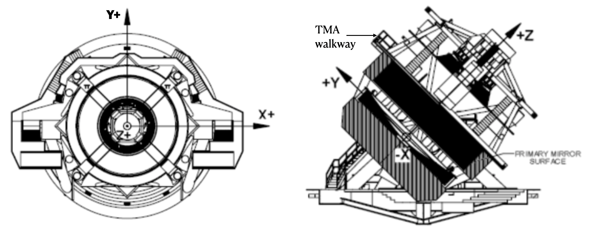
Figure 1 Optical Coordinate System (OCS). Left: view from the sky; Right: side view from the -X axis.
The idea is that the OCS is fixed to M1, which defines the reference for the optical system. Relative to the ground, the OCS rotates with the azimuth angle and the zenith angle. An easy way to identify the +x/+y/+z while looking at a drawing or the actual hardware is that, the walkway on the TMA, above M1M3, is in the +y direction. Otherwise when we go toward horizon it is going to bump into the dome floor.
Note
The Telescope and Site top-level CS document is LTS-136 [5], and the Camera top-level CS document is LCA-280 [7]. Unlike those two documents, we do not define the Observatory Mount CS or the Azimuth CS, because these CSs, as defined by LTS-136 [5] and LCA-280 [7], actually contradict each other, in terms of which axis points north, which points west, etc.
It was agreed that [8] we should always use elevation angle as the input variable to gravity components of the Look-Up Tables (LUTs).
3 Zemax and PhoSim
We discuss the Zemax CS (ZCS) and PhoSim CS (PCS) first, because these are relatively easier to define - they are self-consistent within their own framework. When we say ZCS, we refer to the global CS as used by the official Rubin Observatory optical model. The good news here is that when we worked with the PhoSim team at Purdue on the AOS simulations, we made sure that the PCS conforms to the project standard, at least externally, to the level that we care about while exercising AOS control. So ZCS and PCS are the same CS. We will just refer to it as the ZCS from now on. The ZCS is defined as,
- The origin of ZCS overlaps with OCS origin, i.e., at the theoretical vertex of M1.
- The +z axis of ZCS points from the sky to M1M3. It follows the direction of the incoming on-axis rays. This is opposite of the OCS +z axis.
- The +y axis is the same as OCS +y axis.
- The +x axis is the opposite of OCS +x axis
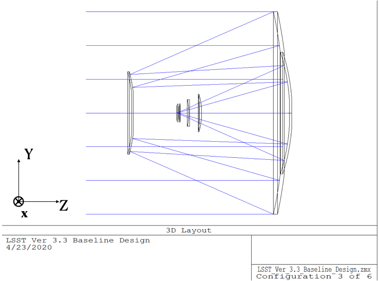
Figure 2 The Zemax/PhoSim Coordinate System (ZCS)
def zcs2ocs(x,y,z):
    return -x,y,-z
def ocs2zcs(x,y,z):
    return -x,y,-z
The optical sensitivity matrix (senM) is derived using the Zemax optical model. Therefore, everything about the senM follows the ZCS. We were able to close the simulation loop with PhoSim, because we made PhoSim consistent with Zemax. With the actual hardware, we will need to convert all commands returned by the AOS control into the proper CS of each component before they are applied.
Note
Note that we apply the decenters and tilts in Zemax via Coordinate Breaks. Mathematically the order of decenters and tilts matter. In Zemax, there is a order flag. When it is set to 0, Zemax does the decenters first, then x-tilt, y-tilt, z-rotation. When the order flag is set to 1, Zemax does these in exact opposite order, so that users can easily go back to the original CS [4]. However, in the AOS context, we don’t really care about these because the tilts are always small enough (on the arc second level) for the order not to make a difference. If this is not true, then the basic approach of taking the decenters and tilts of the hexapods as independent variables in the AOS control wouldn’t be correct.
4 M1M3
The M1M3 glass mirror was casted and polished at the University of Arizona Richard F. Caris Mirror Lab (RFCML). The mirror cell was made by CAID Industries, and software is designed and written by the Rubin Obs. team.
When looking at M1M3 drawings and data, be wary that there are multiple versions of the CSs around. In particular, mechanical folks look at the actuators from inside the M1M3 cell a lot, so they tend to define +z as pointing down from M2. While optical people always look at the M1M3 surface from outside, so they tend to define +z as pointing to the sky. People also flip the +x around the +y axes sometimes. We define M1M3 CS as the following -
- The origin of M1M3 CS overlaps with OCS origin, i.e., at the theoretical vertex of M1.
- +x points toward actuator 106.
- +y points toward actuator 441, which is close to the M1M3 mirror cell door.
- +z points toward the sky.
- When mounted on the TMA, M1M3 CS is the same as OCS.
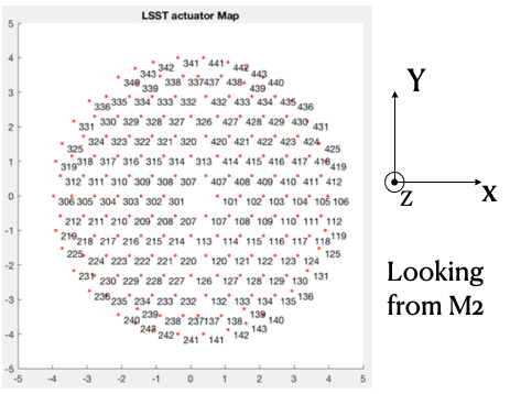
Figure 3 The M1M3 CS.
Our goal here is not to change all the engineering drawings to be in this CS. Instead, the goal is to make sure that for anything that is being used by the AOS, we can put them into M1M3 CS or OCS correctly.
Note that M3 vertex is at (0, 0, -233.8)mm in the OCS.
The Rubin Obs. official M1M3 Finite Element Model (FEM), as provided by Doug Neill and Ed Hileman, uses the M1M3 CS. The bending mode shapes and forces derived using this FEM use the M1M3 CS as well. A visualization of the first 20 M1M3 surface normal bending mode shapes can be found at the bottom of this notebook.
- When the force on an single-axis actuator or the primary cylinder of a lateral or crosslateral actuator is positive, it pushes M1M3 toward the sky, along +z axis. The bending mode forces are given here.
- For bending modes, there are two variaties. The surface normal bending modes are those that were directly measured in the RFCML using the interferometers. Here the displacement vectors of the Finite Element nodes point toward the center of curvature, and are normal to the M1M3 surface. For use in an optical raytrace program like Zemax or PhoSim, and for deriving the senM, we need the surface sag bending modes. These displacement vectors point along +z axis of the OCS or M1M3 CS.
Like other components of the AOS, M1M3 operates mostely off its LUT, which contains our best knowledge of the forces as functions as gravity (or elevation angle) and temperature profiles on and around the mirror surfaces. The current M1M3 LUT can be found here.
- The elevation angle, as the primary input to the M1M3 LUT, is defined the same way as the OCS elevation angle as defined in Sec. 2 The Optical Coordinate System.
- Unrelated to the bending modes, but relevant to the LUT, are the forces on the secondary cylinders of the lateral and crosslateral actuators. The lateral actuators have their secondary cylinders oriented 45 degrees from the +y axis (for +Y laterals) or -y axis (for -Y laterals) in the y-z plane. Their primary use is to support the weight of the mirror for off-zenith pointings and slews in the altitude direction. The cross-lateral actuators have their secondary cylinders oriented 45 degrees from the +x axis (for x<0) or the -x axis (for x>0) in the x-z plane. These are used primarily for azimuth slewing. See all the M1M3 actuator types and their orientations here.
- 96 out of the 100 lateral actuators are +Y laterals. When the force on the secondary cylinder of an +Y lateral actuator is positive, it pushes M1M3 in the y-z plane, along 45 degrees between +y and +z axes.
- 4 of the lateral actuators are -Y laterals (due to space constraints). When the force on the secondary cylinder of an -Y lateral actuator is positive, it pushes M1M3 in the y-z plane, along 45 degrees between -y and +z axes.
- There are 12 crosslateral actuators, 6 on each side of the +y axis. When the force on the secondar cylinder of a crosslateral actuator is positive, it pushes M1M3 in the x-z plane, along the 45 degree line between either the +z and +x (if the crosslateral actuator has x<0) or the +z and -x directions (if the crosslateral actuator has x>0).
The M1M3 control software uses the M1M3 CS as well (see here). When we reposition the M1M3 mirror relative to its cell, that is in referece to the M1M3 CS.
Important
When we derive the senM, we transform M1M3 bending modes into ZCS before applying them in Zemax. Therefore, M1M3 bending mode commands as returned by AOS control is directly applicable to the M1M3 system.
5 M2
The M2 mirror substrate was manufactured by Corning Inc. M2 mirror polishing, mirror cell and control software production were all done at Harris Corporation.
The M2 system as a whole, especially on the software side, leaves a lot to be desired. For example, with regard to the CS, the M2 control software in LabView uses a different CS than the Matlab tools used for generating the configurations.
We define the M2 CS as the following -
- The origin of the M2 CS is on the +z axis of the OCS, and at M2 vertex (6156.201mm from M1 vertex, based on v3.3 optical design).
- The +x axis points toward actuators B8/B9.
- The +y axis points toward tangent link A1 and actuator B1.
- The +z axis points toward the sky.
- When mounted on the TMA, M2 CS has its 3 axes parallel to those of the OCS, all in the same direction. The coordinates of M2 CS origin in the OCS is (0, 0, 6156.201)mm.
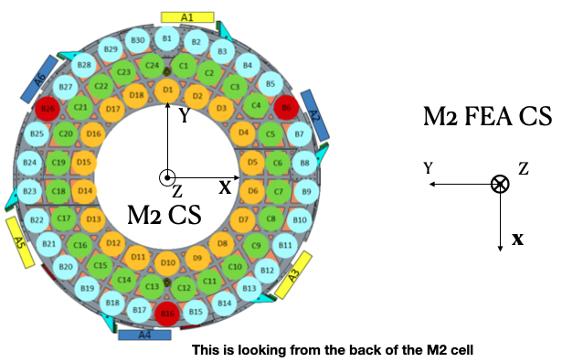
Figure 4 The M2 CS and M2 FEA CS.
#all units are in mm
def ocs2m2cs(x,y,z, d_M2_M1):
    '''
     d_M2_M1 is the distance between M2 vertex and M1 vertex.
          it is approximately 6156.201mm,
          but varies with M2 hexapod positioning and filter band.
    '''
    return x,y,z-d_M2_M1
def m2cs2ocs(x,y,z, d_M2_M1):
    return x,y,z+d_M2_M1
Our goal here is not to change all the engineering drawings to be in this CS. Instead, the goal is to make sure that for anything that is being used by the AOS, we can put them into M2 CS or OCS correctly.
Because we will continue to use the Harris Matlab tools to generate configuration files, for example, when a hardpoint fails and we need to reconfigure a different actuator to work as hard point, we need to define the CS used by the M2 Matlab tools. Since the Harris FEM uses the same CS, and we have been doing Finite Element Analysis (FEA) with it, we call it the M2 FEA CS -
- The origin of the M2 FEA CS overlaps with the M2 CS (at M2 vertex)
- The +y axis points toward actuators B23/B24.
- The +x axis points toward tangent link A4 and actuator B16.
- The +z axis points toward M1M3.
Harris derived a set of M2 bending modes prior to M2 cell and mirror delivery, but those made no sense to us at all. The M2 bending modes that we use now have been calculated by us using the final FEM as delivered by Harris. This FEM uses the M2 FEA CS which we define above. For ease of use, we convert these bending modes into the M2 CS, and make them available here .
def m2fea2m2cs(x,y,z):
    return -y,-x,-z
def m2cs2m2fea(x,y,z):
    return -y,-x,-z
The M2 LabView control software uses M2 CS (most likely by coincidence). See here. The M2 Matlab tools which are used to generate the configuration files uses the M2 FEA CS. See here. The configuration file thus generated are usable by the LabView software because when the configuration files refer to actuators, for example, in the influence matrix and decoupling matrix, they refer to them by actuator IDs instead of their coordinates. When we reposition the M2 mirror relative to its cell, that is in referece to the M2 CS. The axial actuator force distribution found on the M2 Engineering User Interface (EUI) uses the M2 CS.
So, on the bending modes -
- The bending mode forces were calculated in the M2 FEA CS but then converted into the M2 CS. At zenith pointing, a positive bending force means that the actuator is pulling up. While applying the forces to the control system, the forces are also in the M2 CS, where a positive force means pulling the mirror toward the cell, as evidenced in the LUT test.
- To be consistent with M1M3, M2 bending mode shapes also come with two variaties. The surface normal bending modes has the displacement vectors pointing toward the center of curvature of M2 on the back side of M2, and are normal to the M2 surface. The surface sag bending modes have the displacement vectors along +z axis in the M2 CS.
A visualization of the first 20 M2 surface normal bending mode shapes can be found at the bottom of this notebook.
Some clarifications on the M2 LUT -
- As we discussed above, for axial actuators, a positve force always pulls the M2 mirror. That is why during the LUT test, the axial forces went negative when the mirror faced up. The same applies to the tangent links, i.e., the tangent forces are positive when the tangent links pull. That is why during the LUT test, when tangent link A4 was going toward the ceiling, forces on A2 and A3 were positive.
- The elevation angle, as the input variable to the M2 gravity component of the LUT, is in the range of [-270, +90] degrees. This is because that for engineering purposes the M2 mirror needs to rotated on its cart by 360 deg. When the telescope moves from zenith pointing to horizon pointing, the elevation angle goes from 90 degrees to 0.
- The M2 inclinometer read out obeys the same definition as the M2 elevation angle. See here.
Important
When we derive the senM, we transform M2 bending modes from M2CS into ZCS before applying them in Zemax. Therefore, M2 bending mode commands as returned by AOS control are in M2CS and directly applicable to the M2 system.
6 M2 Hexapod
The M2 hexapod was manufactured by Moog CSA Engineering.
The M2 hexapod uses M2 CS. A few additional notes -
- The center of rotation (COR) can be reconfigured with the software, we will set the COR at M2 vertex for AOS operations, so that it overlaps with the origin of M2 CS.
- The +x axis points toward actuator 6.
- The +y axis points toward actuator 1.
- The +z axis points away from the M2 mounting surface.
- Strictly speaking, the order of decenters and rotations matter. However, in the AOS context, we don’t really care about these because the tilts are always small enough for the order not to make a difference.
- When mounted on the TMA, actuator 1 is in the OCS +y direction, actuator 6 is in the OCS +x direction.
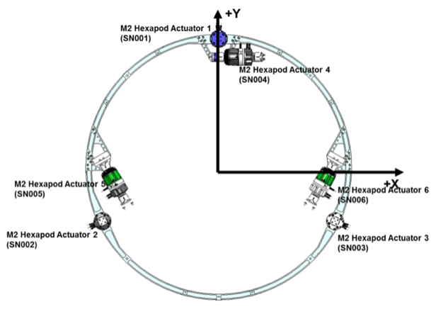
Figure 5 The M2 hexapod in the M2 CS.
The M2 hexapod LUT angle is defined the same way as the OCS elevation angle, ranging between 0 and 90 degrees.
Important
When we derive the senM, we apply the M2 hexapod motions in ZCS. When we use PhoSim to close the simulation loop, PhoSim also interprets those hexapod commands in ZCS. But the actual hardware applies those commands in M2 CS, so we need to convert the commands into M2 CS before they are applied. This transformation can easily be derived using matrix transformations laid out in Document-18499 [9]. For convenience, here we give it more explicitly
# rotation around z-axis (rz) is not needed in AOS control
def zcs2m2cs_cmd(dx, dy, dz, rx, ry):
   return -dx, dy, -dz, -rx, -ry
7 LSSTCam
The Camera Coordinate System (CCS) has been widely used by the Camera team. As pointed out in Sec. 2 The Optical Coordinate System, LTS-136 [5] and LCA-280 [7] actually contradict each other in some aspects. But the good news is that both the Azimuth CS defined by LTS-136 [5] and the Telescope CS defined by LCA-280 [7] have +z pointing toward the sky, and +y pointing at zenith when telescope points at horizon. So the CCS as defined by LCA-280 [7] can be made consistent with our OCS, if we forget about its orientation relative to the earth. (Yes, LCA-280 [7] explicitly uses north and west to define the CCS.)
In the AOS context, we define the CCS as the following (We believe this is the same as the CCS used by the camera team; We redefine it here simply because we find the definition of CCS in LCA-280 [7] rather confusing.)
- The origin of the CCS is at L1S1 vertex. L1S1 is the first surface, i.e., out-facing (away from the rest of the camera) surface of L1. This is about 3397mm from the M1 vertex, based on v3.3 optical design. Note that this distance also varies with the filter band.
- The +z axis points from L1S1 into the camera body, along the optical axis, so that most of the camera components have positive z.
- The +x axis points toward raft R42, along the parallel transfer direction of the individual segments. The segments are roughly 500 by 2000 pixels. The parallel transfer direction is along the 2000-pixel side.
- The +y axis points toward raft R24, along the serial register. The serial register is along the 500-pixel side of the CCD segments.
- When mounted on the telescope mount, with the rotator angle at zero, the x/y/z axes of the CCS are in parallel with the x/y/z axes of the OCS, and points in the same directions.
The CCS is fixed to the camera body; we use the focal plane to define the CCS because that is the only camera component that is relevant to the AOS, CS-wise. The lens surfaces do change under different gravity and thermal profile, and even the camera rotator angle. But the AOS does not actively control any camera internal components for image quality improvements.
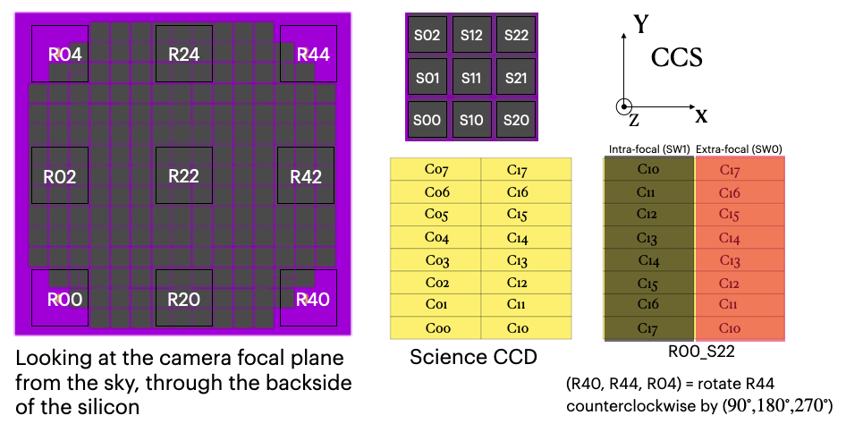
Figure 6 The CCS and orientations of individual CCDs and amplifiers in the CCS.
The orientation of individual CCDs in the CCS is shown in the top of the middle column. Below it we show the layout of the amplifiers for the CCDs. This applies to both e2v and ITL CCDs. Note that a lot of amplifier-level data that are in the camera eTraveller system come as lists, each with 16 elements, one for each amplifier. The ordering is [C10, C11, …, C16, C17, C07, C06, …, C01, C00]. On some camera plots they are labelled as [amp1, amp2, …, amp16].
For the wavefront sensors, the split between the intra- and extra-focal chips are parallel to the CCS y-axis on R00 and R44, and parallel to the CCS x-axis on R40 and R04. Here we refer to each 2k by 4k as one chip. Sometimes we see them refered to as half-chips as well. The one closer to the field center is always the extra-focal chip, which has larger z-coordinate in the CCS. The camera team refers to the extra-focal chip as low chip or SW0 sometimes, because it is lower than the focal plane when looked through the L3 lens. For the same reason, the intra-focal chips are refered to as high chips or SW1. The figure above (bottom right) also shows the naming of the amplifiers on R00_S22. The wavefront sensors at the other three corners are simply rotated versions of R00_22, by \(90^\circ\) (R40_S02), \(180^\circ\) (R44_S00), and \(270^\circ\) (R04_S20).
The official camera detector plane drawing is LCA-13381 [6].
Most of the science sensor segments, as seen in the CCS, has the parallel transfer direction parallel the x-axis. However, astronomers are much more used to seeing images with the parallel transfer direction going vertically, and serial register going horizontally. LSE-349 [3] defines the project’s official Data Visualization CS (DVCS) as a x-y transpose of the CCS. We should be aware that most of the time when we see a visualization of certain quantities over the entire focal plane, a raft, or a single CCD, if the CS is not explicitly given, the assumption should be that it is in DVCS.
# all units are mm
def ocs2ccs(x,y,z, d_L1_M1):
    '''
    d_L1_M1 is the distance between L1S1 vertex and M1 vertex.
         it is approximately 3397mm,
         but varies with camera hexapod positioning and filter band.
    '''
    return x,y,z-d_L1_M1
def ccs2ocs(x,y,z, d_L1_M1):
    return x,y,z+d_L1_M1
def dvcs2ccs(x,y,z):
    return y,x,z
def ccs2dvcs(x,y,z):
    return y,x,z
The wavefront sensors are rotated on the focal plane. The wavefront sensor images we get from the DAQ will need to be rotated to be put into the CCS. See here in the IM code or here in ts_wep code [1] The cwfs code was developed initially for R44. The mask parameter interpolation and off-axis distortion coefficients interpolation were initially modeled for R44 as well. We then rely on the axi-symmetry of the optical system to deal with the other wavefront sensors - we rotate a wavefront sensors by a multiple of 90 degrees to get it to the R44 position, do all the interpolations we need to get proper parameters, then rotate back to its true location.
| [1] | The rotations for the real images from the DAQ may need to be different, because whether or not the DAQ does the rotation for us is TBD. |
When the telescope points at zenith, with zero azimuth angle, the OCS +y will point to south, and OCS +x will point to west. If a source in the sky starts from the bore sight and moves north (increasing Declination), it is going to show up on the detector as moving in +y in the CCS (see off-axis raytrace in the figure below). If a source in the sky starts from the bore sight and moves east (increasing Right Ascension), it is going to show up on the detector as moving in +x in the CCS. Therefore, relative to R22, sources on R44 have larger Ra and Dec values.
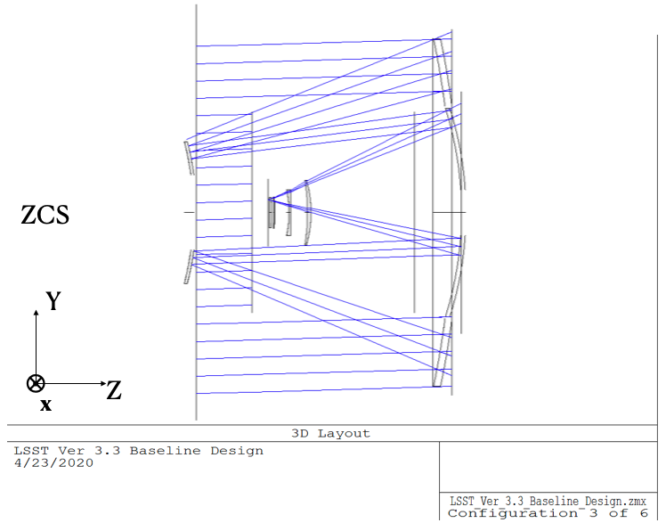
Figure 7 Off-axis rays in the ZCS.
8 Camera Hexapod
The Camera hexapod was manufactured by Moog CSA Engineering.
The Camera hexapod uses the CCS. A few additional notes -
- The center of rotation (COR) can be reconfigured with the software, we will set the COR at L1S1 vertex for AOS operations, so that it overlaps with the origin of the CCS.
- The +x axis points toward actuator 6.
- The +y axis points toward the mid-point between actuators 1 and 2.
- The +z axis points away from the camera mounting surface.
- Strictly speaking, the order of decenters and rotations matter. However, in the AOS context, we don’t really care about these because the tilts are always small enough for the order not to make a difference.
- When mounted on the TMA, actuators 1 and 2 are in the OCS +y direction, actuator 6 is in the OCS +x direction.
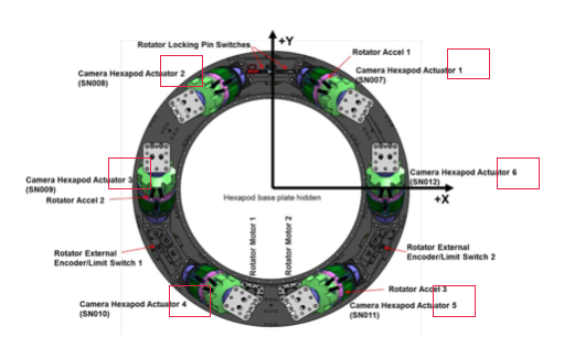
Figure 8 The Camera hexapod in the CCS.
The camera hexapod LUT angle is defined the same way as the OCS elevation angle, ranging between 0 and 90 degrees.
Important
When we derive the senM, we apply the Camera hexapod motions in ZCS. When we use PhoSim to close the simulation loop, PhoSim also interprets those hexapod commands in ZCS. But the actual hardware applies those commands in CCS, so we need to convert the commands into CCS before they are applied. This transformation can easily be derived using matrix transformations laid out in Document-18499 [9]. For convenience, here we give it more explicitly
# rotation around z-axis (rz) is not needed in AOS control
def zcs2ccs_cmd(dx, dy, dz, rx, ry):
   return -dx, dy, -dz, -rx, -ry
9 Alignment Imperfections
Having discussed the M2 CS, the Camera CS, and the hexapods, in this section we talk about what happens when the hexapods are not in perfect alignment.
Fig. Hexapod CS, Camera CS, and Collimated Camera CS. shows how the camera hexapod CS relates to the Camera CS and Collimated Camera CS. We use the hexapod hexapod as the example here. What we discuss below applies to the M2 hexapod as well. When alignment imperfections are taken in account, we need to define a few additional CS to have a clear picture. Otherwise, when a hexapod reports that it is at position (x,y,z,rx,ry,rz), it is not obvious what CS it refers to.
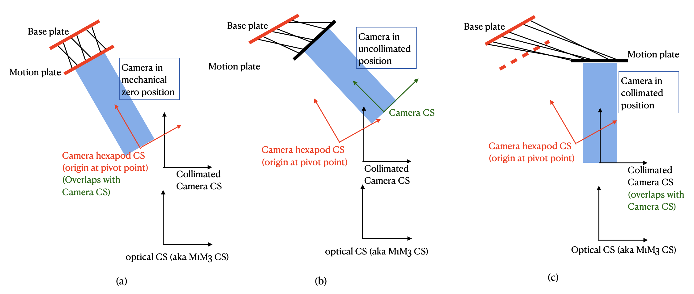
Figure 9 Hexapod CS, Camera CS, and Collimated Camera CS.
The collimated camera CS is the Camera CS when the camera is perfectly aligned. The collimated camera CS is fixed relative to the Optical CS, or M1M3 CS. It does not move with the hexapod.
Due to mechanical imperfections, the base plate of the hexapod will not be in parallel with the xy plane of the collimated Camera CS. When alignments aren’t perfect, the motion plate will not be in parallel with the x-y plane of the collimated Camera CS either. We therefore need to define the camera hexapod CS, which is fixed relative to the base plate. The Camera CS is still the same as defined in Sec. 7 LSSTCam. It is fixed to the camera hardware, therefore also fixed relative to the camera hexapod motion plate.
In Fig. Hexapod CS, Camera CS, and Collimated Camera CS. (a), the camera hexapod is in its mechanical zero position. When the hexapod is in mechanical zero position, the base plate is in parallel with the motion plate. The hexapod actuator encoder readings are at their pre-calibrated offset values. The hexapod control system reports (x=0, y=0, z=0, rx=0, ry=0, rz=0).
The hexapod low-level controller configuration allows users to speicify the position of the pivot point. For AOS operations, we define the pivot point at L1S1 vertex or M2 vertex when the hexapod is in its mechanical zero position. The pivot point, once defined, doesn’t move with the camera or M2. It is fixed relative to the hexapod base plate.
To pivot point configuration interface requires the user to supply (x,y,z) of the pivot point. To understand how to specify the (x,y,z) for the pivot point, or to make sure the current default is what we want, we have to define another CS, which we call the “hexapod pivot CS”. The origin of the hexapod pivot CS is at the center of the telescope-side mounting surface, for both the Camera and M2 hexapods. The z-axis is perpendicular to the telescope-side mounting surface and points toward the sky. The y-axis points to actuator#1 for the M2 hexapod, and to the midpoint between actuator#1 and #2 for the camera hexapod. The x-axis is determined by the right-hand rule. The (x, y, z) used by the pivot configuration is in reference to this CS. Note that Fig. 2 in Sec. 2.2. of LTS-206 has a schematic drawing of this CS, but doesn’t explicitly define the x and y axes.
The positions reported by the hexapod control system and MTHexapod CSC are in the hexapod CS. The Camera hexapod CS is shown in red in Fig. Hexapod CS, Camera CS, and Collimated Camera CS.. The origin of the hexapod CS is at its pivot point. The x, y, and z axes are in parallel with the hexapod pivot CS, which is defined above. The x-y plane is in parallel with the telescope-side mounting surface. The Camera CS overlaps with the hexapod CS when the camera is in its mechanical zero position (Fig. Hexapod CS, Camera CS, and Collimated Camera CS. (a)).
Fig. Hexapod CS, Camera CS, and Collimated Camera CS. (b) shows the camera in a random uncollimated position. Now the camera CS has moved away from the camera hexapod CS, because the camera CS moves with the camera.
In Fig. Hexapod CS, Camera CS, and Collimated Camera CS. (c), the camera is in its collimated position. The camera CS has been moved so that it overlaps with the collimated camera CS. It is clear that the goal of camera hexapod alignment is to position the camera hexapod so that the camera CS overlaps with the collimated camera CS.
For clarify, the hexapod pivot CS is not shown in Fig. Hexapod CS, Camera CS, and Collimated Camera CS.. The difference between the camera mechanical zero position (left) and its collimated position (right) in Fig. Hexapod CS, Camera CS, and Collimated Camera CS. has been greatly exagerated.
10 Camera Rotator
The camera rotator was manufactured by Moog CSA Engineering.
Figure 10 The Camera roator uses the CCS. This is looking at the camera mounting surface from the M1M3.
According to the rotator operator’s manual [2], while looking from the sky, a positive rotation angle is counterclockwise. This is opposite of the azimuth angle as defined in the OCS. In simulations, both PhoSim and the Operation Simulator (OpSim) use the command rotTelPos to define the rotator angle. This angle defines the projection of pupil onto the detectors.
When the telescope points at zenith, with zero azimuth angle, the OCS +y will point to south, and OCS +x will point to west.
Looking from the sky, a positive rotator angle rotates the camera counterclockwise.
The pupil rotation relative to the camera will be clockwise.[2]
| [2] | A related angle as used by the similations is the rotSkyPos, which defines the sky rotation relative to the camera coordinates, i.e. the projection of the sky onto the detectors. We want rotSkyPos to stay constant during tracking. Other things unchanged, looking from the sky, a positive rotator angle makes the sky turn clockwise relative to the camera (north moves toward the east). The corresponds to an increase in rotSkyPos. |
When the rotator angle is non-zero, the CCS is rotated around the optical axis, along with the science sensors and wavefront sensors. But the commands we send to M1M3, M2, and the hexapods will still need to be their own CSs, in order for the commands to be interpreted properly. So we have to de-rotate somewhere in the AOS pipeline. The possible options are -
- Rotate the images (from the CCS into the OCS). This is not a good option - rotating CCD images involves intensity interpolation, which introduces additional noise. For example, astigmatisms have all their signal in the donut boundary, and 200nm of astigmatism only shifts the boundary by about 1/3 pixels. This can easily get lost in image rotation.
- Rotate the senM (so that the Zernikes are still in the CCS while the AOS commands are in the OCS). The senM can be rotated analytically since it is based on an axisymmetric system. Only the Zernikes need to be rotated, in both the orientation (pupil coordinates) and their positions relative to the field center (image coordinates). A function will need to be developed to create a senM in real time using the camera rotation angle as the input. Mathematically this should not be hard to do, but it will be less intuitive for debugging when things go wrong. That is why we prefer the next option, at least during early commissioning. We can reconsider this option after things appear to work correctly with the next option.
- Rotate final AOS commands before they are sent to subsystems. The senM will stay the same. The AOS control, including senM inversion etc. will happen in the CCS. The AOS commands are first determined in the CCS, then rotated into M1M3 CS/OCS (for M1M3), M2 CS (for M2 and M2 hexapod), and CCS (for Camera hexapod).
Note that the AOS actually uses the annular Zernikes. When we say Zernikes we are also referring to the annular Zernikes. More discussions on the (annular) Zernikes are found in Sec. 12 Pupil Coordinates.
import numpy as np
import scipy.interpolate as interpolate
def deRotateBendingModes(coeff, rAngle, mirror):
    '''
    input parameters:
         coeff: the bending mode coefficients in CCS
         rAngle: camera rotator angle, in degrees (counterclockwise when look from the sky)
         mirror: an mirror object, either M1M3 or M2
    output:
        rotated coeff in OCS
    Note: this is proof of concept for now. Since this needs to be done in real time,
        we should store bending modes on a grid, so that we can avoid interpolating
        scattered data all the time. It is slow.
    '''
    nb = len(coeff) #number of bending modes
    nNodes = len(mirror.bx) #number of surface nodes
    z_ccs = np.zeros(nNodes) #surface shape in CCS
    for i in range(nb):
        z_ccs += mirror.bz[:,i]*coeff[i]
    c = np.cos(np.radians(rAngle))
    s = np.sin(np.radians(rAngle))
    x_ocs = mirror.bx*c - mirror.by*s #document-18499 Eq. (9)
    y_ocs = mirror.bx*s + mirror.by*c #x and y in OCS
    f = interpolate.Rbf(x_ocs, y_ocs, z_ccs)
    z_ocs = f(mirror.bx, mirror.by)
    return np.linalg.pinv(mirror.bz).dot(z_ocs)

def deRotateHexapod(cmd, rAngle):
    '''
    input parameters:
         cmd: hexapod command [dz, dx,dy,rx,ry] in CCS, with rx and ry in degrees
         rAngle: camera rotator angle, in degrees (counterclockwise when look from the sky)
    output:
        rotated hexapod cmd in OCS, with rx and ry in degrees
    Note:
        if v1 and v2 are 2 vectors in CS1, and v2 = O v1
           T transforms v1 and v2 into CS2
           (T v2) = (T O T^-1) (T v1)
        see Document-18499 for more details on T and O.
    '''
    [dz, dx, dy, rx, ry] = cmd
    transM = np.array([[1,0,0,dx], [0,1,0,dy], [0,0,1,dz], [0,0,0,1]]) #document-18499, Eq (3)
    c = np.cos(np.radians(rx))
    s = np.sin(np.radians(rx))
    rxT = np.array([[1, 0, 0 ,0], [0, c, -s, 0], [0, s, c, 0], [0,0,0,1]])#document-18499, Eq (5)
    c = np.cos(np.radians(ry))
    s = np.sin(np.radians(ry))
    ryT = np.array([[c, 0, s ,0], [0, 1, 0, 0], [-s, 0, c, 0], [0,0,0,1]]) ##document-18499, Eq (7)
    O = transM.dot(rxT).dot(ryT)
    c = np.cos(np.radians(rAngle))
    s = np.sin(np.radians(rAngle))
    T = np.array([[c, -s, 0,0], [s,c,0,0], [0,0,1,0], [0,0,0,1]]) ##document-18499, Eq (9)
    mm = T.dot(O).dot(np.linalg.inv(T))
    print(mm)
    # we can analytically do transM*rxT*ryT on paper, then match matrix elements to mm above.
    # transM * rxT * ryT =
    # [c_ry,      0,    -s_ry,      dx],
    # [-s_rx*s_ry,0,    -s_rx*c_ry, dy],
    # [c_rx*s_ry, s_rx, c_rx*c_ry,  dz],
    # [0,         0,      0,         1]
    [dx, dy, dz] = mm[:-1,-1]
    rx = np.degrees(np.arcsin(mm[2,1]))
    ry = np.degrees(np.arcsin(-mm[0,2]))
    return dz, dx, dy, rx, ry

def deRotateCmd(aos_cmd_ccs, rAngle, M1M3, M2):
    '''
    input parameters:
         aos_cmd_ccs: aos commands determined in CCS. This is a 50x1 vector, ordered as
                 [M2 hexapod (dz, dx, dy, rx, ry), Camera hexapod (dz, dx, dy, rx, ry),
                    M1M3 bending modes 1-20, M2 bending modes 1-20]
         rAngle: camera rotator angle, in degrees (counterclockwise when look from the sky)
         M1M3 and M2: mirror objects, with bending mode data
    output:
        aos commands which have been transformed into OCS
    '''
    m2_hex = aos_cmd_ccs[:5]
    cam_hex = aos_cmd_ccs[5:10]
    m1m3_bm = aos_cmd_ccs[10:30]
    m2_bm = aos_cmd_ccs[30:50]
    m1m3_bm_ocs = deRotateBendingModes(m1m3_bm, rAngle, M1M3)
    m2_bm_ocs = deRotateBendingModes(m2_bm, rAngle, M2)
    m2_hex_ocs = deRotateHexapod(m2_hex, rAngle)
    cam_hex_ocs = deRotateHexapod(cam_hex, rAngle)
    return np.hstack((m2_hex_ocs, cam_hex_ocs, m1m3_bm_ocs[:20], m2_bm_ocs[:20]))
11 ComCam
The ComCam is a one-raft camera that will be used in commissioning. In terms of pixel coordinates, ComCam uses the CCS as its standard CS. As the hardware and optics are a bit different from the LSSTCam, we define the ComCam CS (CCCS) as the following -
- The origin of CCCS is on L1S1 vertex of ComCam. This is different from the L1S1 vertex of the LSSTCam. Therefore the CCCS is shifted along z relative to the CCS. According to the as-built ComCam optical model, L1S1 is about 4108mm from the M1 vertex. Note that this distance also varies with the filter band.
- The +x points toward sensor S21, along the parallel transfer direction of the individual segments. The segments are roughly 500 by 2000 pixels. The parallel transfer direction is along the 2000-pixel side.
- The +y axis points toward sensor S12, along the serial register. The serial register is along the 500-pixel side of the CCD segments.
- The +z points into the ComCam body, and toward the sky.
The definition of CCCS origin above implies that when the ComCam is mounted on the TMA, the camera hexapod will use ComCam L1S1 as its COR. Alternatively we could still set the COR at the imaginary LSSTCam L1S1 vertex, which would enable us to compare the tilt angles to the hexapod positioning accuracy, repeatability, and range requirements directly. We choose ComCam L1S1 vertex mostly because the PhoSim ComCam model has this implemented as the COR for the hexapod. And we need PhoSim to close the ComCam AOS loop in simulation mode. Due to the lack of PhoSim support, we try to avoid changing the COR in PhoSim. Also note that when we close AOS loop with ComCam we would have already verified all the requirements on the subcomponents, and we can convert a tilt in the CCCS into the CCS easily, if needed.
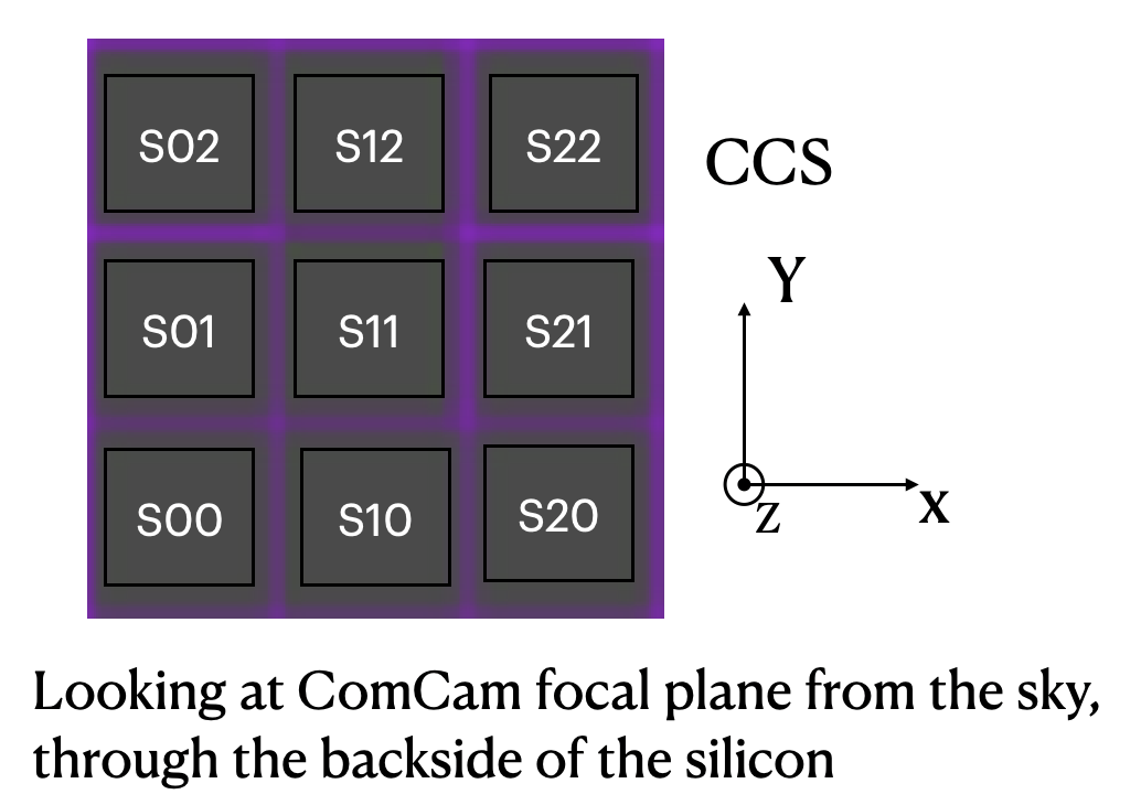
Figure 11 The ComCam CS in the same as CCS in pixel coordinates.
# all units are mm
def ocs2cccs(x,y,z, d_CCL1_M1):
    '''
    d_CCL1_M1 is the distance between ComCam L1S1 vertex and M1 vertex.
         it is approximately 4108mm,
         but varies with camera hexapod positioning and filter band.
    '''
    return x,y,z-d_CCL1_M1
def cccs2ocs(x,y,z, d_CCL1_M1):
    return x,y,z+d_CCL1_M1
12 Pupil Coordinates
Because the senM is calculated in ZCS, the annular Zernikes we use in conjunction with the senM also need to be in the ZCS. Assuming the images we get from the DAQ is in CCS, we need to convert them into ZCS before we run cwfs on them. Since from CCS to ZCS is a 180 degree rotation around the y-axis, the images simply need a left-right flip.
import numpy
def ccs2zcs_img(img):
     return numpy.fliplr(img)
When the images are in ZCS, the output annular Zernikes as measured by cwfs are also in ZCS. Our definition of the annular Zernike polynomials follows Ref. [10], which reduces to the original Noll Zernikes [11] when the obscuration ratio approaches zero. Zemax [4] uses the same annular Zernike definitions.
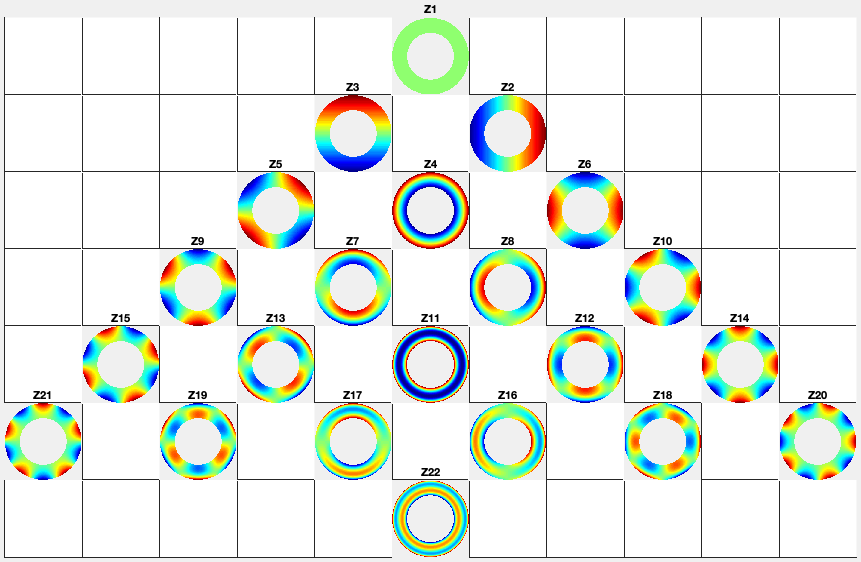
Figure 12 The Annular Zernike polynomials.
It is also worth mentioning that, by convention (see [1], for example), longer optical path length (OPL) means larger phase delay, and the optical path difference (OPD) is negative. For example, in the Zemax model,
- if we put on a phase screen with 2 waves of z4 (focus) at the entrance pupil, it means 2 waves of phase delay, where the edge of the pupil is delayed more than the center. The wavefront is going to show -2 waves of z4. The effect is like M1 curvature of radius is increased (M1 is more flat). The intra focal image gets larger.
- If we put on a phase screen with 2 waves of z5 (45 deg astigmatism) at the entrance pupil, the wavefront is going to show -2 waves of z5. The OPL is longer (OPD is more negative) along the 45 degree line. The effect is like M1 has been pulled back along the 45 degree line, into a potato-chip shape. The image is more elongated along the 45 degree line.
Note
Ideally we want the senM and the Zernikes to be all in CCS, in which case we can largely forget about ZCS. We are keeping them in ZCS for now, because if we switch everything to CCS then the current closed-loop simulations with PhoSim will break (or at least require non-trivial work to add additional CS transformations in order to maintain convergence.) Once everything works smoothly with the real hardware, we will reconsider converting senM and the Zernikes into CCS. It won’t be hard to do, because, for example, an astigmatism with any orientation can be decomposed into z5 and z6, same for the coma pair, trifoid pair, and so on.
13 Alignment System
The way the Alignment System Control (ASC) works is to measure the rigid body positions of M2 and the camera in the M1M3 CS or some CSs that are tied to the M1M3 CS, determine the offset relative to their reference positions, then command the hexapods to move M2 and the camera to their reference positions.
To facilitate the above operations, it would be the easiest to have the ASC report target positions in the M2 CS and CCS, for M2 and the camera, respectively, so that the inverse of the offsets can be sent to the hexapods without further coordinate transformations. After a command is issued to measure the position of a target (M2 or Camera), a measurement plan is executed by the Spatial Analyzer (SA), which measures the x, y, and z of all the Spherically Mounted Reflectors (SMSs), and fit them to an internal model of the target. The CSs used by the SA are configurable.
The SMRs for the camera will rotate with the rotator. The SA can measure the rotation angle and take that into account when reporting the camera position. The reported camera position will be the same as what one would get by setting roator angle to zero and doing the same measurement.
14 Summary
To summarize, to operate the AOS properly, we will have to continue to use the following CSs,
- ZCS (same as PCS)
- OCS
- M1M3 CS
- M2 CS
- M2 FEA CS
- CCS and CCCS (with zero rotator angle)
- CCS and CCCS (with non-zero rotator angle)
The document intends to capture the definitions of these CSs, and the transformations between them. As we go further into testing and commissioning, it may become clearer that there are better ways to handle particular aspects of these CS definitions and transformations. The document is expected to be a living document and be updated when design decisions change.
References
| [1] | Applied Optics and Optical Engineering, Volume XI, volume 11, January 1992. |
| [2] | Moog CSA Engineering. LSST Rotator Operator’s Manual. Moog CSA Engineering, CSA report No. OM-7403-101, 2018. |
| [3] | [LSE-349]. K. Simon Krughoff. Defining the Transformation Between Camera Engineering Coordinates and Camera Data Visualization Coordinates. 2019. URL, https://ls.st/LSE-349. |
| [4] | (1, 2) Radiant Zemax LLC. ZEMAX Optical Design Program User’s Manual. Radiant Zemax LLC, 2013. |
| [5] | (1, 2, 3, 4, 5) [LTS-136]. D. Neill and J. Sebag. Telescope OptoMechanical Coordinate Systems. 2011. URL, https://ls.st/LTS-136. |
| [6] | [LCA-13381]. Martin Nordby. LSST Camera Detector Plane Layout. 2020. URL, https://ls.st/LCA-13381. |
| [7] | (1, 2, 3, 4, 5, 6, 7) [LCA-280]. Martin Nordby and John Ku. LSST Camera Mechanical Standards. 2013. URL, https://ls.st/LCA-280. |
| [8] | [SITCOMTN-004]. B. Xin. Implementation of the rubin aos luts. 2020. URL: http://SITCOMTN-004.lsst.io |
| [9] | (1, 2, 3) [Document-18499]. B. Xin and G. Angeli. LSST Coordinate Systems. 2015. URL, https://ls.st/Document-18499. |
| [10] | Virendra N. Mahajan. Zernike annular polynomials for imaging systems with annular pupils. Journal of the Optical Society of America A, 1(6):685, June 1984. doi:10.1364/JOSAA.1.000685. |
| [11] | R. J. Noll. Zernike polynomials and atmospheric turbulence. Journal of the Optical Society of America (1917-1983), 66:207–211, March 1976. |
| [12] | J. R. Peterson, J. G. Jernigan, S. M. Kahn, A. P. Rasmussen, E. Peng, Z. Ahmad, J. Bankert, C. Chang, C. Claver, D. K. Gilmore, E. Grace, M. Hannel, M. Hodge, S. Lorenz, A. Lupu, A. Meert, S. Nagarajan, N. Todd, A. Winans, and M. Young. Simulation of Astronomical Images from Optical Survey Telescopes Using a Comprehensive Photon Monte Carlo Approach. \apjs , 218:14, May 2015. arXiv:1504.06570, doi:10.1088/0067-0049/218/1/14. |